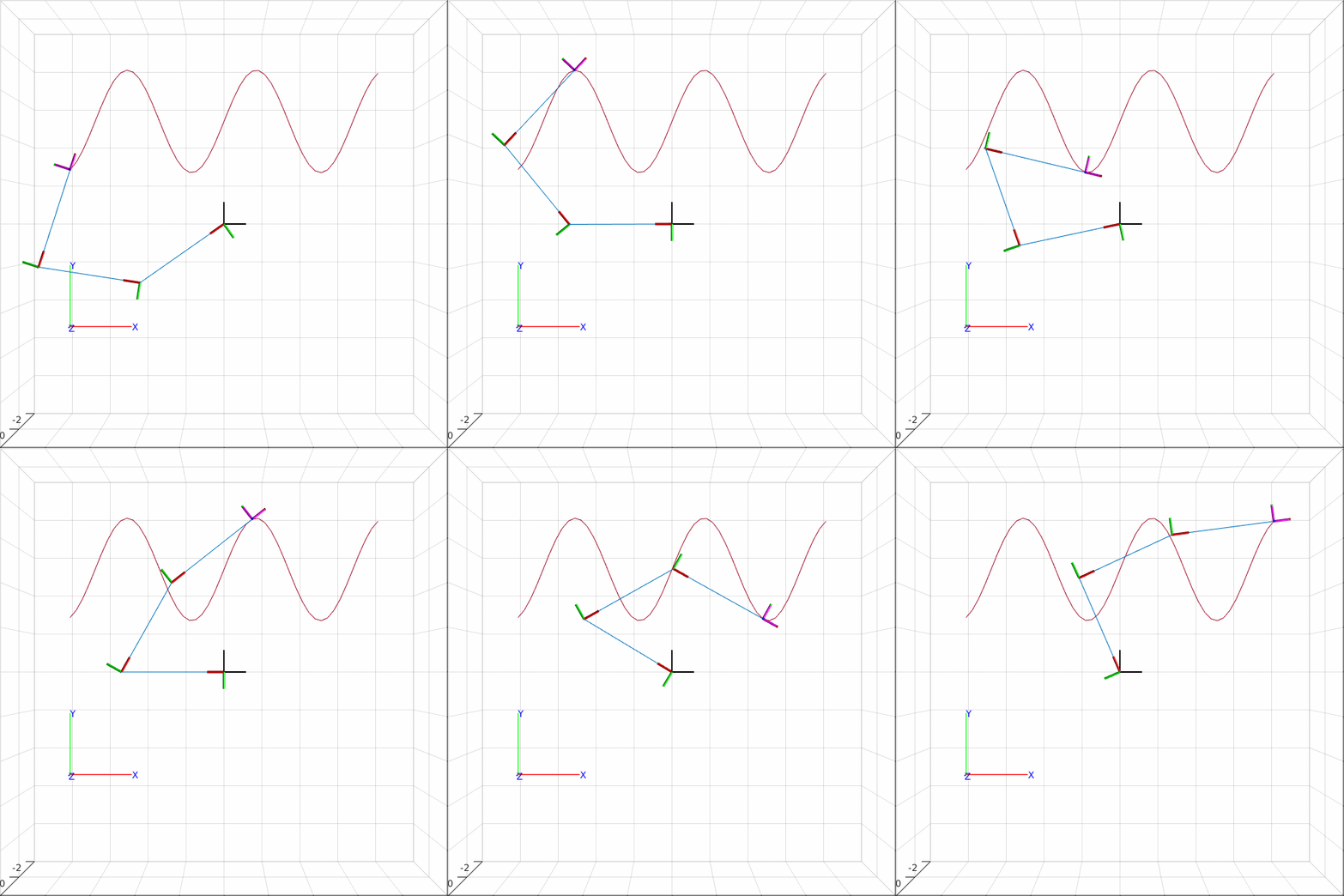
Controlling 3R planar robot
In my last post I showed how to build a 3R planar robot using the MATLAB robotics system toolbox (RST).
In this post I will show you can perform forward and inverse kinematics for the robot. Lastly we will make the robot’s end effector follow a sine wave. This tutorial is based on MATLAB’s 2-D Path Tracing With Inverse Kinematics example.
Forward kinematics
Forward kinematics is about finding the end effector position and orientation given a set of joint angles $q$. Position and orientation are the components of a pose, which can be represented in a homogenous transformation matrix $T \in R^{4x4}$. We write the forward kinematics of a robot as $T(q)$. The structure of $T$ is as follows:
\[\mathbf{T}=\left[\begin{array}{cc} \mathbf{R} & \mathbf{p} \\ \mathbf{0}_{1 \times 3} & 1 \end{array}\right]\]$p$ is the positional displacement of the frame, while $R$ is a 3x3 orthogonal matrix belonging to the special orthogonal group $SO(3)$. This basically means that multiplying two matrices in $SO(3)$ will yield a new matrix also in $SO(3)$. $R$ describes the orientation of the frame.
In a matlab prompt we write the following code. Note that build_3R_robot is simply all the commands from the previous post put into a function.
>> robot = build_3R_robot;
>> robot.getTransform([0 0 0]', 'ee_link')

ans =

    1.0000         0         0    1.5000
         0    1.0000         0         0
         0         0    1.0000         0
         0         0         0    1.0000
In this case we supplied $q = [0,0,0]^T$ and since each link is 0.5m long, we get that the end effector frame is displaced 1.5m along the x-axis. The rotational part is the identity matrix corresponding to zero rotation.
Inverse kinematics
Given a pose $T$, inverse kinematics (IK) seeks to find the joint angles that places the robot end effector in this pose. In general there are two methods for solving the IK problem.
- Find a closed form inverse kinematics solution. For a 6 degree of freedom (DOF) robot, there will usually be 8 solutions corresponding to left/right-handed, elbow up/down and wrist flipped/not flipped. For a redundant manipulator there are infinitely many solutions and we should instead:
- Use a numerical iterative approach typically called Iterative Inverse Kinematics. Matlab uses the latter method.
In the following code, we create an inverseKinematics object - this object can solve the inverse kinematics problem. We also create a transformation matrix $T$ with a displacement of 1.5m along x. Notice this is the same $T$ as the one we found with forward kinematics.
>> ik = inverseKinematics('RigidBodyTree', robot);
>> T = transl(1.5,0,0);
>> ik('ee_link', T, [0 0 0 1 1 1], robot.randomConfiguration)

ans =

   -0.0024
    0.0062
   -0.0051
We query for a solution by using ik(endEffectorName, pose, weights, qStartGuess). The endEffectorName is the name of the last link, in this case ‘ee_link’. The weights correspond to how important it is for the rotation and position to achieve the exact pose. In the function call above [0 0 0 1 1 1] means we do not care about the orientation. An iterative inverse kinematics solver always needs a start guess - preferably a good one (meaning the robot is already close to the desired pose). In this case I use a randomConfiguration.
Notice that the answer is not $q = [0,0,0]^T$ as we would expect - but it is quite close. This is the nature of a numerical approach.
Tracing a sine wave path

A path is a list of poses that we wish to achieve to have the end effector achieve. The following code starts by loading the robot object and creating the inverse kinematics solver. Then we produce a stack of poses. The poses all have zero rotation, but the translational component traces out a sinewave. We perform inverse kinematics for each pose.
Since there are infinitely many solutions for a 3R planar robot in the plane, we help the robot by updating the start guess. This makes it more likely that we get solutions that lie close to each other. It is however evident from the GIF above, that all is not perfect. As the robot reaches the second wave peak it makes a large skip - this is not ideal as we would probably not be able to reproduce this movement on a real robot.
%% Load robot and create IK solver
robot = build_3R_robot;
ik = inverseKinematics('RigidBodyTree', robot);

%% generate poses:
x = linspace(-0.75,0.75,50);
y = 0.5 + 0.25*sin(10*x);
z = zeros(1, length(x));

t = [x', y', z'];
poses = transl(t);

%% Perform inverse kinematics for each pose
qs = zeros(50,3);
qGuess = robot.randomConfiguration
for i = 1:length(poses)
    T = poses(:,:,i);
    q = ik('ee_link', T, [0 0 0 1 1 1], qGuess);
    qs(i,:) = q';
    qGuess = q;
end

%% Visualize:
[positions] = transl(poses)
plot(positions(:,1)', positions(:,2)')
axis([-1 1 -1 1])
view(2);
hold on

for i = 1:length(qs)
    q = qs(i,:)';
    robot.show(q, 'PreservePlot', false);
    drawnow
end
Finally we visualize the robots movement:
